OmicsNet has been developed to allow researchers to easily create and visualize multi-omics networks from
one or more list(s) of molecules of interests identified from a multi-omics study such as mRNAs, proteins, miRNAs, transcription factors, metabolites, SNPs, LC-MS peaks,
as well as microbiome taxa. The networks can be explored in a three-dimensional (3D) space and conventional 2D visualization.
In particular:
From a list (or multiple lists) of molecules of interest (mRNAs, transcription factor, miRNA, microbial taxa, metabolites or even MS peaks) to molecular
interaction networks using build-in comprehensive knowledge base.
Visual exploratory analysis of the network in our innovative 3D network visualization system with rich features for
layout, coloring, highlighting, functional and topological analysis.
Some example visualization results can be seen from our Overview page.
OmicsNet version 2 has been updated to enable researchers to integrate less well established omics data including LC-MS peaks from untargeted metabolomics, microbial taxa from microbiome surveys,
as well as SNPs. In details,
Users could upload a list of LC-MS peaks (in csv or txt format). The predicted potential metabolites and their corresponding chemical artifacts (e.g. adducts, isotopes)
will be annotated and predicted directly.
Microbiome survey data (taxon list) are also supported to integrate with other omics data through their potential metabolic products based on genome-scale metabolic models (GEMs);
Single nucleus polymorphisms (SNPs) data through their associated mRNAs based on either positional mapping or eQTL results.
Molecular Lists: The format is such that the first column takes the input type and the second column takes the expression value or any other quantitative measurement. Multiple
ID types are supported for different organisms.
List of 691 DE mRNAs from helminth infection signature (download)
Data from multi-omics (transcriptomics, metabolomics) study to identify biomarker of intrahepatic cholangiocarcinoma cancer (ICC)
LC-MS Peak List: OmicsNet accepts MS peaks from LC-MS based untargeted metabolomics studies (formatted as csv or txt). The data list consists of four columns (m/z, RT, intensity and P value, sequentially).
The first three columns are mandatory, while P values column is optional. If no p value provided, all annotated compounds will be included for network construction.
Network Files: three different formats are supported including .json, .sif, .txt and .graphml format.
Please click on the following links to see example files supported:
The 3D visualization system was developed based on the Web Graphics Library or WebGL technology.
WebGL is the standard 3D graphics API for the web. It allows developers to harness the full power of the computer’s 3D rendering hardware
from within the browser using JavaScript. Before WebGL, developers had to rely on plugins or native applications and ask their users to
download and install custom software in order to deliver a hardware-accelerated 3D experience.
WebGL is supported by most major modern browsers that support HTML5. We have tested OmicsNet in several major browsers (see below).
Our empirical testings have shown that Google Chrome usually gives the best performance for the same computer:
In the System section, ensure the Use hardware acceleration when available
checkbox is checked (you'll need to relaunch Chrome for any changes to take effect)
Then enable WebGL:
Type chrome://flags in the browser and press Enter
Ensure that Disable WebGL is not activated
(you will need to relaunch Chrome for any changes to take effect)
Here you will have to change Default to Enabled in the drop down.
Type about:config in the browser address bar and press enter
Search for webgl.disabled
Ensure that its value is false (any changes take effect immediately without relaunching Firefox)
Then inspect the status of WebGL:
Go to about:support
Inspect the WebGL Renderer row in the Graphics table:
If your graphics card/drivers are blacklisted, you can override the blacklist.
Warning: this is not recommended! (see blacklists note below). To override the blacklist:
OmicsNet builds interaction networks starting from list(s) of input molecules: mRNA/protein, TF, miRNA, metabolite, and supports the integration
of multiple interaction types. OmicsNet can also process and integrate list of microbial taxa, peaks generated from untargeted metabolomics and SNPs to the molecular interaction framework.
The workflow can be dissected in four steps:
Upload list(s) of input molecules.
Select interaction database and compute individual omics interaction networks using input list(s) and/or predicted interacting partners from primary interaction network.
Merge interaction networks identified from second step into connected subnetworks, perform network trimming and filtering (optional).
Network visual analysis in 2D or 3D space.
There are three main scenarios of network building:
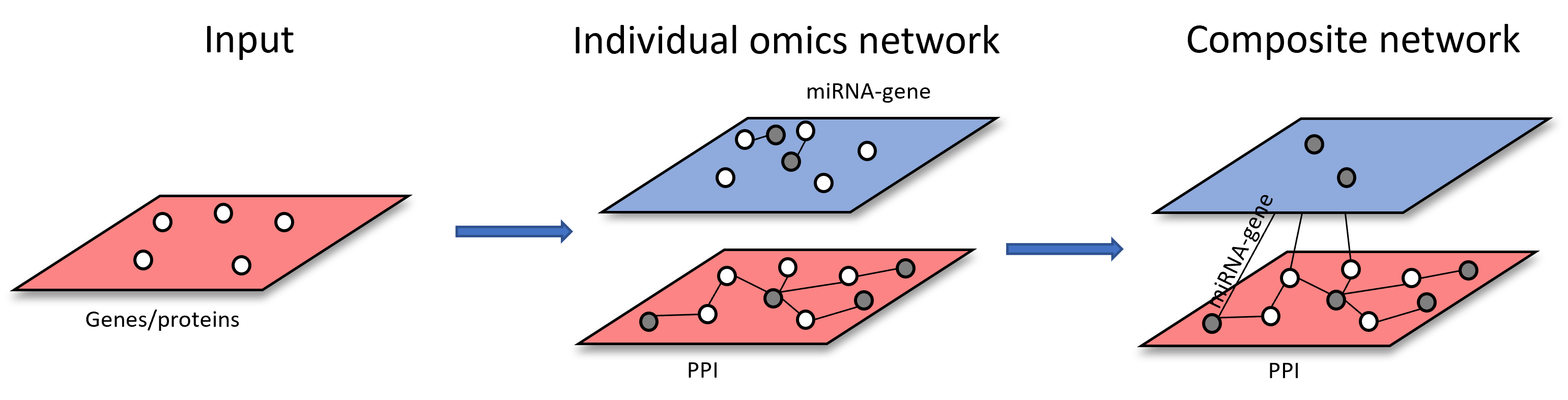
Scenario 1: upload a list of omics features and search against different interaction databases using the seed features from list upload as query. An example of network construction starting from gene list is shown below:
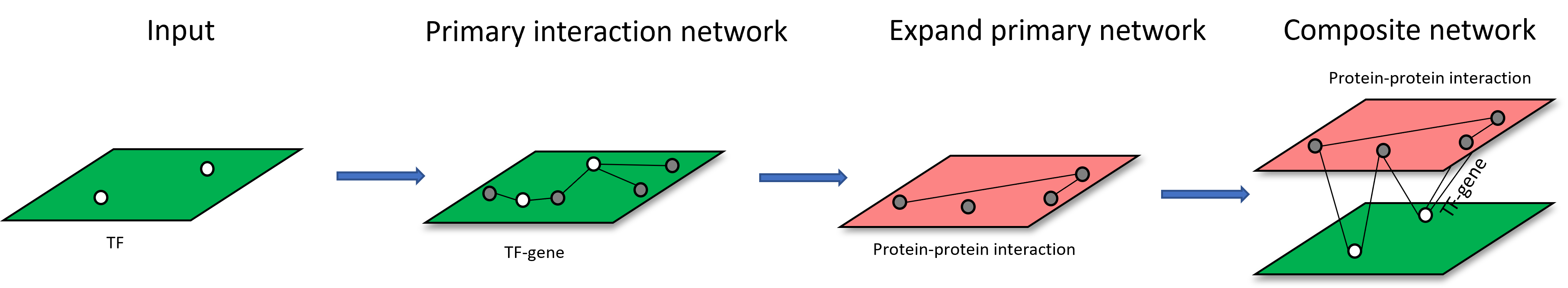
Scenario 2: upload a list of omics features, build a primary interaction network and expand the primary interaction networks by adding other types of interactions by using nodes from primary interaction network as query.
An example of network construction starting from TF list is shown below:
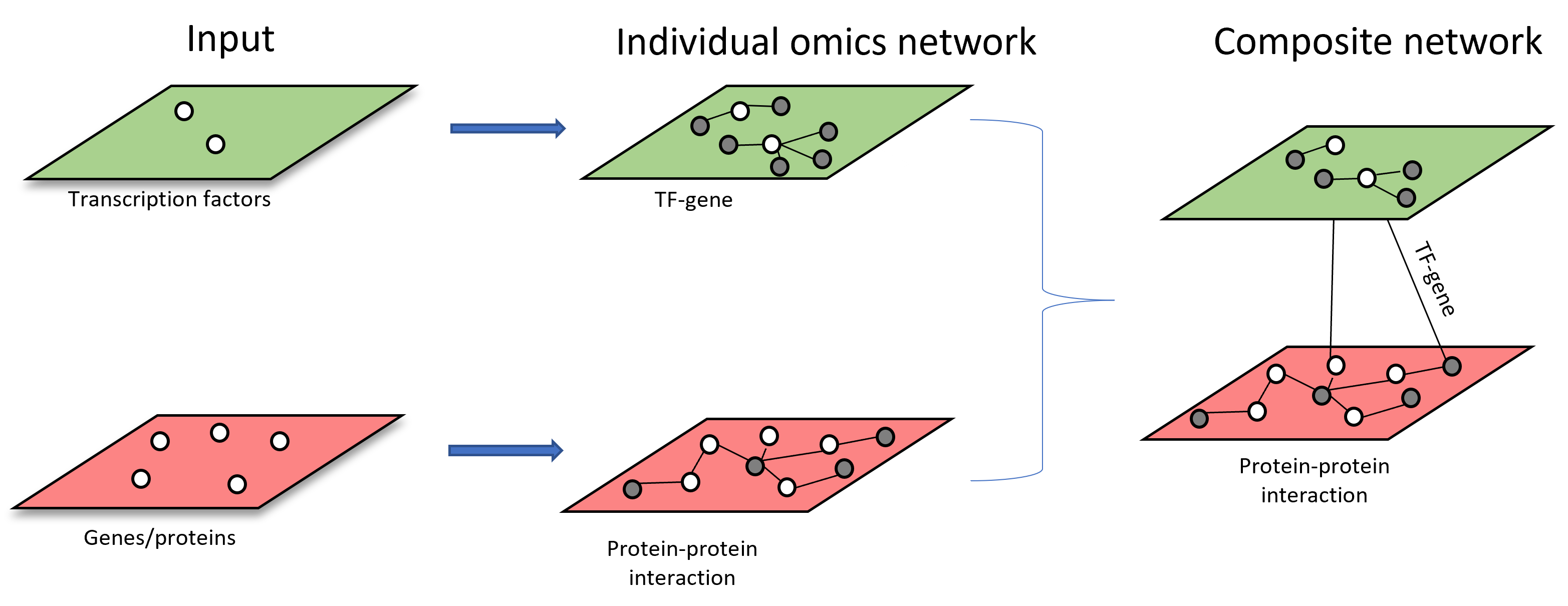
Scenario 3: starting from more than one types of omics features. Each list of omics features will be used to build individual omics interaction networks.
The resulting individual networks will be merged through shared nodes to form multi-omics network (i.e. Metabolite-protein and metabolite-taxa networks are merged through shared metabolites across both networks)
The above approaches will typically return one giant subnetwork ("continent") with multiple smaller ones ("islands").
Most subsequent analyses are performed on the continent. Note, networks with less than 3 nodes will be excluded.
This error is usually encountered when the seed molecules themselves are not found within the selected interaction type and the primary interaction network has not been created yet.
For instance, uploading list of SNPs, it is required to first query "SNP-mRNA" database before querying any other types of interactions (Protein-protein, Metabolite-protein, etc).
OmicsNet uses high-quality protein-protein interaction (PPI) data from STRING. database, the most comprehensive PPI database to date. This database collects
and integrates already published experimental data on PPI in addition to predicted interactions. A filter can be applied to subset higher confidence
interactions based on STRING provided combined score of confidence and whether the interactions have experimental evidence. Our human PPI database
contains around 670 000 interactions while our mouse database contains around 900 000 interactions. To supplement human and mouse data, we also provide
PPI data from InnateDB, a database built by manual curation from published literature as well as experimental data from several PPI databases including
IntAct, MINT, DIP, BIND and BioGRID.
JASPAR: Database of transcription factor binding motifs. The TF-gene information is obtained by using position weight matrices
of transcription factors binding preferences are used to scan the promoters
of all mRNAs present in the range of 500 bp upstream to 2000 bp downstream of a transcription factors start site.
For a mRNA to be considered as targeted by a transcription factor, a 100% match to consensus sequences of the promoter
must be obtained through the scan. Mice data are derived from human data.
ENCODE: Transcription factor target data derived from ENCODE Chip-seq data. We performed an initial filter to keep peak signal with score above 500 only and performed TF targets prediction on the binding data using BETA minus
algorithm. It outputs a regulatory potential score based on the over-representation and distances between the binding sites
and mRNA transcription start site within a range of genomic region. An average of the regulatory scores are taken for targets
if more than one experiment is done on the same TF. We applied a filter to only include TF targets having a regulatory score
more than 1. Please refer to BETA paper for more information on mRNA matching. Mice data are derived from original experiments
performed on mouse tissues or cells.
Wang, Su, et al. "Target analysis by integration of transcriptome and ChIP-seq data with BETA." Nature protocols 8.12 (2013): 2502-2515.
The data is from miRNet which has collected data mainly from miRTarBase and TarBase. Both databases curate their experimentally validated
microRNA-target interactions from the literature. For humans, we have around 330 000 interactions involving
2596 different miRNAs. For mice, there are around 58 000 interactions involving 769 miRNAs.
Metabolite-protein interaction data were obtained from Recon 2 for human. Recon 2 is one of the most complete metabolic
reconstruction of human metabolism. This model was built by a community of domain experts which aggregates information
from cell type/organ specific metabolic reconstructions such as HepatoNet1, literature and previous knowledge bases such
as Recon 1 and EHMN (Edinburgh Human Metabolic Network).
KEGG: species-specific metabolite-protein interaction data derived from KEGG reference reactions by mapping these
reference reactions to species-specific and reaction-specific enzymatic proteins and metabolites.
VEP: The Ensembl Variant Effect Predictor(VEP) is a powerful toolset for the analysis and annotation of genomic variants which provide
access to an extensive collection of genomic annotation.
It distinguish from other approaches by aiding prioritization of variants across transcripts and manage the complexities of variant analysis.
Two major sources, GENCODE and
Reference Sequence (RefSeq) at the National Center for Biotechnology Information (NCBI),
are used for Homo sapiens annotation.
Based on VEP annotation mapping to the latest GRCh38 human assembly, we provide a configurable flank ranging from 5000 to 50000 base
pairs to search for overlaps between input variants and genomic features. User can either choose a specific distance or the nearest few
mRNAs to generate the manageable SNP-mRNA interaction network.
PhenoScanner: a curated database of publicly available results from large-scale genetic association studies in humans. It currently contain
over over 150 million genetic variants and
about 84 million associations with mRNA expression. Variants annotation will be performed using Ensembl Variant Effect Predictor V88 with GENCODE
transcripts V26 mapped to build 37 positions. The nearest mRNAs for intergenic variants were retrieved using the
BEDOPS tool version 2.4.26. Expression quantitative trait loci (eQTLs)
analysis is important for understanding the effect of SNPs on mRNA expression.
The original association database was calculated for all the pairs within 500 Kb, while to produce manageable results on our website, only results
with P < 1 * 10-5 (suggested by the original study) are returned for queries SNPs.
ADmiRE: Annotative Database of miRNA Elements(ADmiRE) dedicate to miRNA variant annotation which combines multiple existing and new
biological annotations of variation in miRNAs across human datasets.
10,206 mature (3,257 within seed region) miRNA variants annotated from multiple large sequencing datasets such as gnomAD (15,496 genomes;
123,136 exomes) are included.
SNP2TFBS: a database essentially provide specific annotations for human SNPs, namely whether they are predicted to abolish, create or change the affinity of one or several transcription factor (TF) binding sites.
A SNP's effect on TF binding is estimated based on a position weight matrix (PWM) model for the binding specificity of the corresponding factor.
TFBSs from the JASPAR database are used to generate the SNP-Tf asscociations. For each SNP it provides the list of TFBSs (PWMs) affected, sorted by the magnitude of the effects.
MS peaks are firstly annotated once uploaded into OmicsNet. The annotation algorithm is developed and evolved from NetID (PMID: 34711973).
The whole process includes 5 steps:
MS Peak Import: MS peaks from users' uploading is recognized and cleaned. All MS signals meeting the ppm criteria and RT difference less
0.5% of the whole RT range will be merged as a single peak. All database and analyzing elements are loaded in this step;
MS Data Pre-processing: All MS peaks are potentially matched towards HMDB database and annotated as multiple chemical identities basically;
Besides, the intuitive relationships among the annotated peaks are found to establish a minimal network;
Network Propagation: The network generated by the previous step will be propagated in this step. This propagation is trying to find out more
associations among the nodes (peaks) as well as more potential chemical identities for each nodes. Twice bio-transformation together with three time
abiotic propagation are performed;
Global Network Optimization: The propagated network from last step is organized as a huge but sparse constraint matrix; The matrix is maximized
with integer linear programming powered by lpsymphony package. As a result, only one chemical
identity (node) and more confident bio-/abiotic relationship (edge) are kept;
Annotation and Network Construction: The annotation results are being summarized in this step. Simultaneously, the network (for integration with
other omics data) are filtered based on the p value cut-off of users' input.
When network is too large, interpretation and visualization become difficult. OmicsNet offers various options for reducing the network size.
To compute the minimum network connecting the seed entities. In filter menu, select "Minimum Network" for shortest path based approach or "Steiner Forest(PCSF)" for Prize-Collecting Steiner Forest approach.
To filter the networks to remove undesired nodes based on betweenness and degrees.
To delete promiscuous nodes use filter by degree or remove manually in Network Viewer.
To remove specific nodes and/or edges, use our browse feature in "Database Selection" page. Click on browse button of corresponding interaction network to visualize the network in the browser.
Use advanced filter options for batch removal of nodes or edges in the new window.
To use "Extract Module" function located in the bottom of toolbar to build a subnetwork using an arbitary list of nodes
in the current network.
To reduce the input features by using larger fold change and/or smaller p value cutoffs before uploading your input lists;
In "Database Selection" page, click on "Browse" button of corresponding interaction network and in the new page, delete select interactions by clicking on "Delete" of corresponding rows or use "Advanced filter" for batch removal of nodes and edges.
Genome-scale metabolic models (GEMs) are reconstructions of the metabolic networks of many kinds of cells that computationally describe all
information of an organism including its known genes, the enzymes encoded and associated expression rules (mRNA-protein-reaction, GPR, rules),
and participating metabolites.
It can serve as a scaffold for multi-omics data integration and be used to predict genotype-phenotype relationships in biological systems.
Our tool mainly leverages GEMs of human gut microbes from two databases AGORA(assembly of gut organisms through reconstruction and analysis)
and EMBL GEMs(European Molecular Biology Laboratory).
Agora is a collection of GEMs for 818 human gut microbes, the detailed reconstruction method can be found Stefanía Magnúsdóttir, et al..
EMBL GEMs are built for all reference and representative bacterial genomes of NCBI RefSeq (release 84) using CarveMe(Daniel Machado, et al.), 1288 of which are annotated as human gut microbes.
Potential score describe the probability of a given taxon to produce a given metabolite estimated by corresponding logit regression model. For each metabolite in the selected GEMs resources,
Bayesian logit regression models are trained for each taxonomy level from phylum to strain using the taxon labels in the selected taxonomy level and the origin (whether human gut microbe or not) as predictors.
The predictive result of a input taxon list by the corresponding regression models can be summarized as a matrix with rows as the input taxon and column as the metabolites they can potentially produce complemented by the probability termed as potential score.
Models trained by taxonomy levels with higher resolution tend to present better performance in prediction based on the 10-Fold Cross-Validation and ROC analysis.
A potential score over 0.5 indicates the taxon is more likely to produce the given metabolite and the increasing score value means the greater production possibility.
Potential score is suitable for the comparison of differentiated metabolic functions among different taxa and this method has been successfully applied to microbial tryptophan metabolites prediction(Yao Lu, et al.).
For integrating microbial taxa into the molecular interaction knowledge framework, OmicsNet uses metabolic potential score derived from genome-scale metabolic models (GEMs) and use the predicted metabolites as an entry point.
By default, the primary interaction network is generated by taking as input the resulting predicted metabolites from taxa input and search for other metabolites directly interacting with them (through metabolic reactions).
The interaction data itself also comes from microbial metabolic reactions data extracted from Agora and EMBL GEMs. In the network, the size of metabolite nodes (yellow) represent the number of microbes that are predicted
metabolize it. By clicking on the node, you can see the corresponding microbial taxa and their potential scores. Also, you can visualize the heatmap overview of microbial metabolic potential by clicking on
icon located in the vertical toolbar.
Yes. OmicsNet would automatically annotate all potential abiotic components related with liquid chromatography coupled mass spectrometry, including adducts, isotopes,
in-source fragments, oligomers, heterodimers, ring artifacts, multicharges.
The visualization is limited by the performance of users' computers and screen resolutions.
Too many nodes and edges will result in greater latency in manipulating the network and more severe "hairball" effect.
Based on empircal tests, we have set the maximum number of nodes to 10000. We recommend limiting the total number of nodes to between 200 ~ 2000 for best experience.
For very large networks, please make sure you have a decent computer equipped with a performant graphics card.
To deal with "hairball effect" associated with larger networks, OmicsNet offers several options that can partially address this problem.
Reducing the opacity of edges reduces edge occlusion problem. In Edge Style drop-down menu, select Opacity option.
Use edge-bunding algorithm to deform and aggregate closely located edges to provide a less cluttered view of the network. It is also located in the Edge Style
menu.
If it is a composite network(i.e. multiple types of nodes), apply the 2D perspective multi-layered view to separate molecular types by layer.
Click on icon located in the vertical toolbar.
When uploading list of molecules, an optional second column can be included to add expression value information. In the network visualization page, display
the expression profile by clicking on "Expression" in View drop-down menu.
The connections between nodes of a biological network are not random.
Modules refers to parts of the network that have higher connections within than the average connections
expected across the whole network. It is especially an important aspect of biological network as it can
help in identify nodes that are likely to participate in the same biological function as they are more
likely to be tightly connected as a subgroup of the network.
OmicsNet currently uses three different module detection algorithms including Walktrap, InfoMap and Label Propagation. WalkTrap exploits the idea that random walking tends to remain in a dense part of network which corresponds to a module.
InfoMap algorithm joins neighboring nodes into modules and these modules are further merged into supermodules using the map equation principle.
The map equation minimizes the steps needed for random walker to describe a network by finding network modules. Label Propagation works
by labeling nodes with unique labels at the initial step and, subsequently, nodes take the label that most of its neighbors have until
a consensus label is reached for all nodes. There is no clear advantage on using one algorithm over another, users are welcome to try all three.
In the network generated by OmicsNet, the size of the nodes are based on their degree values, with a bigger size indicating larger degrees.
The color indicates the type of nodes.
To change the layout, please go to the menu bar located on top of network viewer and click on "Layout" dropdown menu to show options including defaut force-directed, hierarchical, layered and spherical layouts.
The layered mode improves the visualization of composite networks where there are multiple interaction types.
It is a variant of standard force directed layout in which graph communities the nodes from a same graph community
are more tightly clustered together forming clusters of nodes. To distinct visually the graph communities, nodes from
the same community are colored the same and a transluscent spheres are added. Double-clicking an individual module or selecting it within module table will put it into the view focus.
You can change the color and size of a node. The shape cannot be changed in the current implementation.
To change the node color, you can use our "Coloring Option" panel to change node color based on
its source molecule type. To change node size, you can keep clicking it (double-clicking) to increase its size. You can also use the
Node Size functions to increase or decrease size of all nodes.
To modify an individual node, you can use our "Modify Node" panel located at the bottom left size of the window. You can either manually
enter the ID of the node to be modified or, on the graph, right click on the node of interest and click on "Modify Node" option from the context menu.
The nodes can be colored based on degree, betweenness, centrality, expression (user-supplied), etc.
To do so, click on Global button in Coloring Options panel located on the top left corner. In the opened window, select
an attribute for which the nodes will be colored in the drop-down menu.
A selection of color schemes are offered from which users can choose from as well.
The node sizes can be scaled based on degree, betweenness, centrality, expression (user-supplied), etc. The default node sizes are scaled by node degrees.
To do so, click on Size option from the Node Style drop down menu. In the opened window, select
an attribute in the drop-down menu from which the size will be scaled to.
Yes, OmicsNet allows users to freely choose the background color. Users can click on the background of "Coloring Options" panel
located on the top left corner of the screen or go to Style menu to select the color..
To drag a single node, simply hold down left click boutton and drag and drop the node to new position.
To drag a group of nodes (2D viewer only), make sure to highlight the group of nodes that are to be moved then
in "Select" menu and go to Scope submenu to select the option
Highlighted. Then drag and drop one of the highlighted features to the new position.
Right click node and select Add Label option from the context menu.
2D Viewer
Nodes will be automatically labeled when their sizes reach a certain threshold. Therefore,
you can simply increase node size to label any node. To do so:
Label a single node: right click a node and choose "Add Label" option in the context menu.
Label all highlighted nodes: use the Node tab in the Display Options panel on top right,
select "Highlighted nodes" and "Increase ++", then keep clicking Submit button to
increase the size until labels show up.
Labels can be hidden and their color can be changed in the Style menu.
To highlight nodes are from input list, please click on highlight seed nodes icon located
in the vertical tool bar located on the top left corner of Network Viewer. To change the halo color, use the color picker located on the top of tool bar.
The default behavior of OmicsNet is highlighting by color for the selection of features from enriched pathways, detected modules and double click. To use
halo highlight effect instead, click on More Options and go to Highlight tab to select Halo Effect Only.
Yes. To do this, first select or highlight section of the network, then go to Module Extraction tab in Advance Options (3D Viewer) or click the
Extract
icon on the left tool bar in the network view of window (2D Viewer). The operation is
expensive, and you have to wait a few seconds for the extracted network to return.
The returned network will be named as "moduleX" and is available in the "Network Explorer"
panel on the top-left of the page for future reference.
Note: 2D viewer is more adapted for manual selection of nodes for the purpose of node extraction. 3D depth perspective make node selection a tedious process.
This process is similar to the Steiner Tree problem where the algorithm identifies a minimal subnetwork containing
all the terminal nodes (highlighted nodes) from the complete network (the current subnetwork). We implemented a heurisitc approach
that provides an approximate answer to this problem to reduce computation time.
By default, there is a fog effect in the scene to accentuate the depth effect of 3D network. To turn off this effect, click on Fog located on the vertical toolbar.
Node-link diagram often suffers from "hairball effect" visual clutters due to large amount of nodes and edges.Edge bundling improved the
readability of such network by using a process analogous to bundling network cable wires. To perform edge bundling click on
located in the vertical toolbar.
Due to the nature of untargeted metabolomics, it covers all chemical components in your sample, including known compounds (shown as KEGG ID), ambiguous knowns and unknowns.
The Network Visualization page displays both known and ambiguous compounds and filters out all unknowns. The ambiguous compounds (also known as putative compounds) are displayed
as molecular formula. They are usually novel compounds that have not been identified.
Yes, you can test enriched gene ontologies or pathways (KEGG/Reactome) for only your query genes.
To do so, first select and highlight query genes using the Highlight Color toolbar on the top
left (you may have to highlight twice for upregulated and downregulated genes respectively); or you can use the
Hub Explorer and select queries from the node table. After that, select a functional catergory
from the Function Explorer section, and click the Submit button.
Yes. Users can perform enrichment tests on currently highlighted nodes in the network. There are two different ways to highlight nodes
Module highlight: perform module detection and select a module on the table.
Manual highlight: select nodes from the data table on the left or by double clicking nodes. Select a "Include eighbours" highlight scope
in "Select" menu to to highlight node and its immediate neighbours.
After you have selected the nodes or modules, click the Perform Enrichment Analysis
button. The result table will be displayed in the panel below. Note, enrichment analyses are
performed on ALL currently highlighted nodes. To ensure only your current selections
are being used, first Reset the network, then perform highlighting/selections before performing
the enrichment analysis.
The enrichment analysis is to test whether any functional modules (gene sets) from the user selected library
are significantly enriched among the currently highlighted nodes within the network. OmicsNet uses
hypergeometric tests to compute the enrichment p values. Note that in the current implementation, enrichment
analysis only takes into account gene/proteins in the network, not the other types of molecules.
Both approaches uses Over Representation Analysis (ORA) approach, however the input genes are different in each case. "Enrichment Analysis" uses all genes or metabolites uploaded by the user while "Functional Explorer" uses
genes present in the current interaction network. ORA on interaction network (Functional Explorer) has the effect of amplifying biological signal by including direct interacting partners of seed molecules in the analysis.
Guilt-by-association approach assumes that genes with similar functions are close to each other in molecular interaction network.
In OmicsNet, we use a Random Walk With Restart (RWR) algorithm to explore the network vicinity of seed nodes and
identify candidate genes that are close to them. The result will output a list of candidate genes with their associated score.
Processing ....
Your session is about to expire!
You will be logged off in seconds.
Do you want to continue your session?
We use cookies.
Essential session cookies are required for the site to function.
Google Analytics
is used to understand website traffic.
 icon on the left tool bar in the network view of window (2D Viewer). The operation is
expensive, and you have to wait a few seconds for the extracted network to return.
The returned network will be named as "moduleX" and is available in the "Network Explorer"
panel on the top-left of the page for future reference.
icon on the left tool bar in the network view of window (2D Viewer). The operation is
expensive, and you have to wait a few seconds for the extracted network to return.
The returned network will be named as "moduleX" and is available in the "Network Explorer"
panel on the top-left of the page for future reference.
 located on the vertical toolbar.
 located in the vertical toolbar.
